library(ggplot2)
library(ggrepel)
library(dplyr)
library(colorspace)
library(tidyverse)
library(readxl)
library(cowplot) # plot_grid
library(scales)
library(corrplot)
library(ggmosaic) # 모자이크와 트리맵|
|
Final Exam
0.1 패키지 불러오기
1 데이터 불러오기
- 1998년 ~ 2023년 4월 국내에서 개봉한 영화
- 독립/예술 영화가 아닌 일반영화 (해외+국내영화)
- 1위 ~ 500위
movie <- read_xlsx('C:/Users/seong taek/Desktop/3-1 DataVisualize/data_visualize/역대 박스오피스2.xlsx')
#> New names:
#> • `` -> `...5`
#> • `` -> `...7`
movie
#> # A tibble: 500 × 11
#> 순위 영화이름 개봉일 매출액 ...5 관객수 ...7 스크…¹ 국적
#> <dbl> <chr> <dttm> <dbl> <chr> <dbl> <chr> <dbl> <chr>
#> 1 1 명량 2014-07-30 00:00:00 1.36e11 <NA> 1.76e7 <NA> 1587 한국
#> 2 2 극한직업 2019-01-23 00:00:00 1.40e11 <NA> 1.63e7 <NA> 1978 한국
#> 3 3 신과함께-… 2017-12-20 00:00:00 1.16e11 <NA> 1.44e7 <NA> 1912 한국
#> 4 4 국제시장 2014-12-17 00:00:00 1.11e11 <NA> 1.43e7 <NA> 966 한국
#> 5 5 어벤져스:… 2019-04-24 00:00:00 1.22e11 <NA> 1.39e7 <NA> 2835 미국
#> 6 6 겨울왕국 2 2019-11-21 00:00:00 1.15e11 <NA> 1.37e7 <NA> 2648 미국
#> 7 7 아바타 2009-12-17 00:00:00 1.28e11 <NA> 1.36e7 <NA> 912 미국
#> 8 8 베테랑 2015-08-05 00:00:00 1.05e11 <NA> 1.34e7 <NA> 1064 한국
#> 9 9 괴물 2006-07-27 00:00:00 0 <NA> 1.30e7 S 167 한국
#> 10 10 도둑들 2012-07-25 00:00:00 9.37e10 <NA> 1.30e7 <NA> 1072 한국
#> # … with 490 more rows, 2 more variables: 국적2 <chr>, 배급사 <chr>, and
#> # abbreviated variable name ¹스크린수1.1 전처리
movie <- movie %>% select(-c(5,7,10))
movie %>% head()
#> # A tibble: 6 × 8
#> 순위 영화이름 개봉일 매출액 관객수 스크…¹ 국적 배급사
#> <dbl> <chr> <dttm> <dbl> <dbl> <dbl> <chr> <chr>
#> 1 1 명량 2014-07-30 00:00:00 1.36e11 1.76e7 1587 한국 (주)씨…
#> 2 2 극한직업 2019-01-23 00:00:00 1.40e11 1.63e7 1978 한국 (주)씨…
#> 3 3 신과함께-죄와 벌 2017-12-20 00:00:00 1.16e11 1.44e7 1912 한국 롯데쇼…
#> 4 4 국제시장 2014-12-17 00:00:00 1.11e11 1.43e7 966 한국 (주)씨…
#> 5 5 어벤져스: 엔드… 2019-04-24 00:00:00 1.22e11 1.39e7 2835 미국 월트디…
#> 6 6 겨울왕국 2 2019-11-21 00:00:00 1.15e11 1.37e7 2648 미국 월트디…
#> # … with abbreviated variable name ¹스크린수movie$국적 %>% unique()
#> [1] "한국" "미국" "일본" "영국" "중국" "프랑스"2 상위5위 & 하위5위 그래프
- 전처리
movie_rank <- movie %>%                       # 0값이 아닌것만 필터링
  select(영화이름, 관객수) %>%         # 열 지정 선택
  mutate(popratio = 관객수/median(관객수)) %>% # 새로운 컬럼 'popratio'
  arrange(desc(popratio)) %>%                      # 내림차순 정렬
  mutate(index = 1:n(),
         label = ifelse(index<=5 | index > n()-5 | index==median(index), 영화이름,''))
# index값이 5이하, 행의 수에서 5를 뺀 값보다 크거나, index가 중위수인 index이면 '행정구역.시군구.별' 값을 가지고 그렇지 않으면 ''(빈문자열) 값 가짐

movie_rank %>% head()
#> # A tibble: 6 × 5
#>   영화이름             관객수 popratio index label
#>   <chr>                 <dbl>    <dbl> <int> <chr>
#> 1 명량               17613682     5.65     1 "명량"
#> 2 극한직업           16264944     5.22     2 "극한직업"
#> 3 신과함께-죄와 벌   14410754     4.62     3 "신과함께-죄와 벌"
#> 4 국제시장           14257115     4.57     4 "국제시장"
#> 5 어벤져스: 엔드게임 13934592     4.47     5 "어벤져스: 엔드게임"
#> 6 겨울왕국 2         13747792     4.41     6 ""
2.1 상위5위 & 하위5위 시각화
ggplot(movie_rank, aes(x = index, y =관객수)) +
  geom_hline(yintercept = 1, linetype = 2, color = 'grey40') +
  geom_point(size = 1, color = 'royalblue')  +
  geom_text_repel(aes(label = label),
                  min.segment.length = 0,
                  max.overlaps = 100) +
  scale_y_continuous(name = '관객수',
                     breaks = seq(1000000, 20000000, by = 2000000),
                     labels = scales::comma_format()(seq(1000000, 20000000, by = 2000000))) +
  scale_x_discrete(name = '관객수 상위5위 & 하위5위 ',
                   breaks = NULL) +
  theme_light() +
  theme(panel.border = element_blank())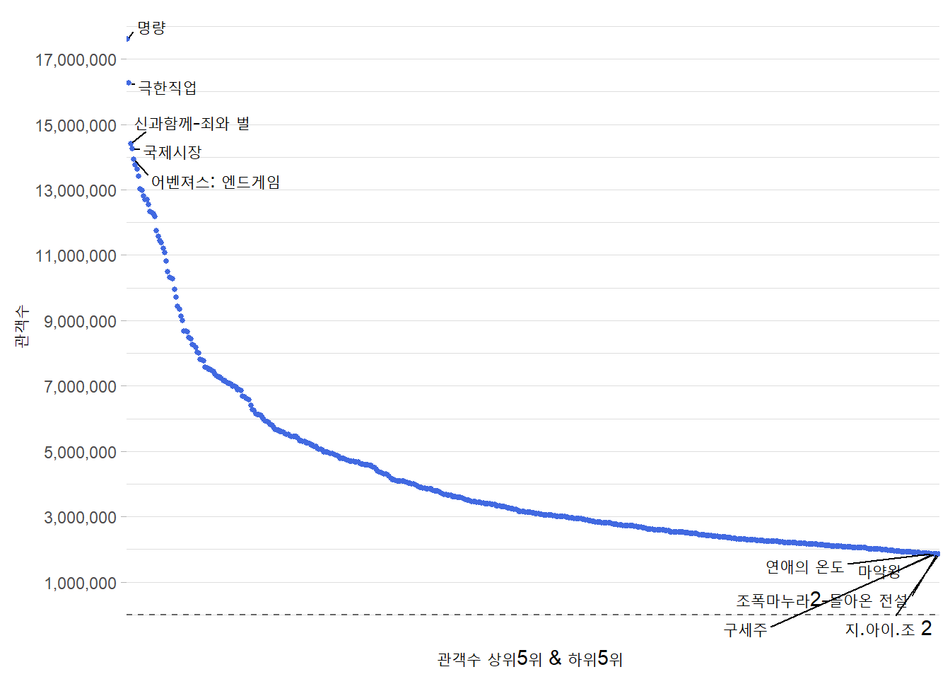
3 매출액 TOP10 영화
- 전처리
movie_rank_sales_10 <- movie %>% arrange(-매출액) %>% slice_head(n=10)
movie_rank_sales_10
#> # A tibble: 10 × 8
#> 순위 영화이름 개봉일 매출액 관객수 스크…¹ 국적 배급사
#> <dbl> <chr> <dttm> <dbl> <dbl> <dbl> <chr> <chr>
#> 1 2 극한직업 2019-01-23 00:00:00 1.40e11 1.63e7 1978 한국 "(주)…
#> 2 25 아바타: 물의 길 2022-12-14 00:00:00 1.38e11 1.08e7 2809 미국 "월트…
#> 3 1 명량 2014-07-30 00:00:00 1.36e11 1.76e7 1587 한국 "(주)…
#> 4 13 범죄도시2 2022-05-18 00:00:00 1.31e11 1.27e7 2498 한국 "주식…
#> 5 7 아바타 2009-12-17 00:00:00 1.28e11 1.36e7 912 미국 "주식…
#> 6 5 어벤져스: 엔드… 2019-04-24 00:00:00 1.22e11 1.39e7 2835 미국 "월트…
#> 7 3 신과함께-죄와 … 2017-12-20 00:00:00 1.16e11 1.44e7 1912 한국 "롯데…
#> 8 6 겨울왕국 2 2019-11-21 00:00:00 1.15e11 1.37e7 2648 미국 "월트…
#> 9 4 국제시장 2014-12-17 00:00:00 1.11e11 1.43e7 966 한국 "(주)…
#> 10 14 알라딘 2019-05-23 00:00:00 1.07e11 1.26e7 1311 미국 "월트…
#> # … with abbreviated variable name ¹스크린수3.1 매출액 TOP10 영화 시각화
sales_top10_plot <-
ggplot(movie_rank_sales_10, aes(x=매출액, y=fct_reorder(영화이름, 매출액))) +
  geom_point(color = "#0072B2", size=4) +
  scale_x_continuous(name = "총 매출액",
                     limits = c(100000000000,160000000000),
                     expand = c(0,0),
                     labels = function(x) paste0(x / 1e+8, "억")) +
  scale_y_discrete(name=NULL, expand = c(0, 0.5)) +
  theme_minimal() +
  theme(plot.margin = margin(18, -15, 3, 1.5))

sales_top10_plot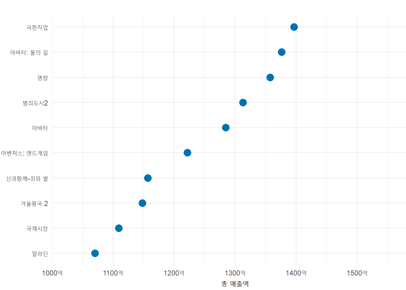
4 관객수 대비 매출액 TOP10
- 전처리
movie_rank_sales_10_contr <- movie %>%
mutate(관객수대비매출액 = (매출액/관객수)) %>%
arrange(-관객수대비매출액) %>% slice_head(n=10)
movie_rank_sales_10_contr
#> # A tibble: 10 × 9
#> 순위 영화…¹ 개봉일 매출액 관객수 스크…² 국적 배급사 관객수…³
#> <dbl> <chr> <dttm> <dbl> <dbl> <dbl> <chr> <chr> <dbl>
#> 1 25 아바타… 2022-12-14 00:00:00 1.38e11 1.08e7 2809 미국 "월트… 12739.
#> 2 311 토르: … 2022-07-06 00:00:00 2.95e10 2.72e6 2143 미국 "월트… 10862.
#> 3 43 탑건: … 2022-06-22 00:00:00 8.79e10 8.18e6 1975 미국 "롯데… 10744.
#> 4 88 닥터 … 2022-05-04 00:00:00 6.26e10 5.88e6 2691 미국 "월트… 10646.
#> 5 325 드래곤… 2010-05-20 00:00:00 2.75e10 2.60e6 562 미국 "유니… 10550.
#> 6 434 블랙 … 2022-11-09 00:00:00 2.22e10 2.11e6 2571 미국 "월트… 10545.
#> 7 147 더 퍼… 2023-01-04 00:00:00 4.79e10 4.59e6 1023 일본 "(주)… 10426.
#> 8 258 이터널… 2021-11-03 00:00:00 3.17e10 3.05e6 2648 미국 "월트… 10402.
#> 9 487 헤어질… 2022-06-29 00:00:00 1.97e10 1.90e6 1374 한국 "(주)… 10369.
#> 10 13 범죄도… 2022-05-18 00:00:00 1.31e11 1.27e7 2498 한국 "주식… 10344.
#> # … with abbreviated variable names ¹영화이름, ²스크린수, ³관객수대비매출액4.1 관객수 대비 매출액 TOP10
- 시각화
sales_top10_cont_plot <-
ggplot(movie_rank_sales_10_contr, aes(x=관객수대비매출액, y=fct_reorder(영화이름, 관객수대비매출액))) +
  geom_point(color = "#0072B2", size=4) +
  scale_x_continuous(name = "1인당 매출액",
                     limits = c(10000,14000),
                     expand = c(0,0),
                     labels = function(x) paste0(x / 1e+0, "원")) +
  scale_y_discrete(name=NULL, expand = c(0, 0.5)) +
  theme_minimal() +
  theme(plot.margin = margin(18, -20, 3, 1.5))

sales_top10_cont_plot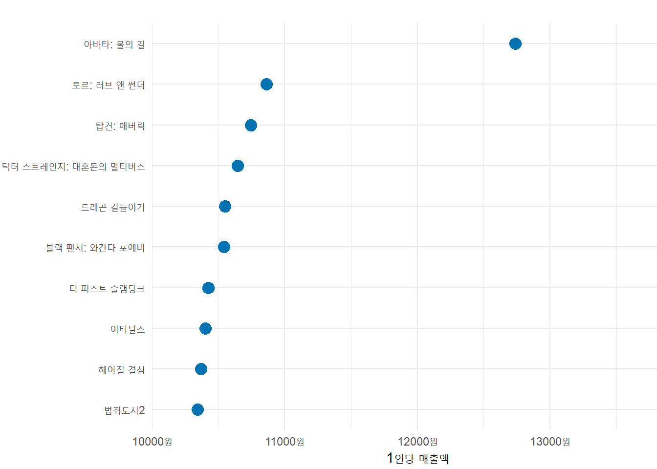
### 2개의 매출액 통계 그래프
plot_ab <- plot_grid(sales_top10_plot,
                     sales_top10_cont_plot,
                     nrow= 1,            # 행의 개수
                     rel_widths= c(3,3), # 각각의 너비
                     labels= c('총 매출액 TOP10 영화',
                               '관객수 대비 매출액 TOP10 영화')) # 라벨 a,b

plot_ab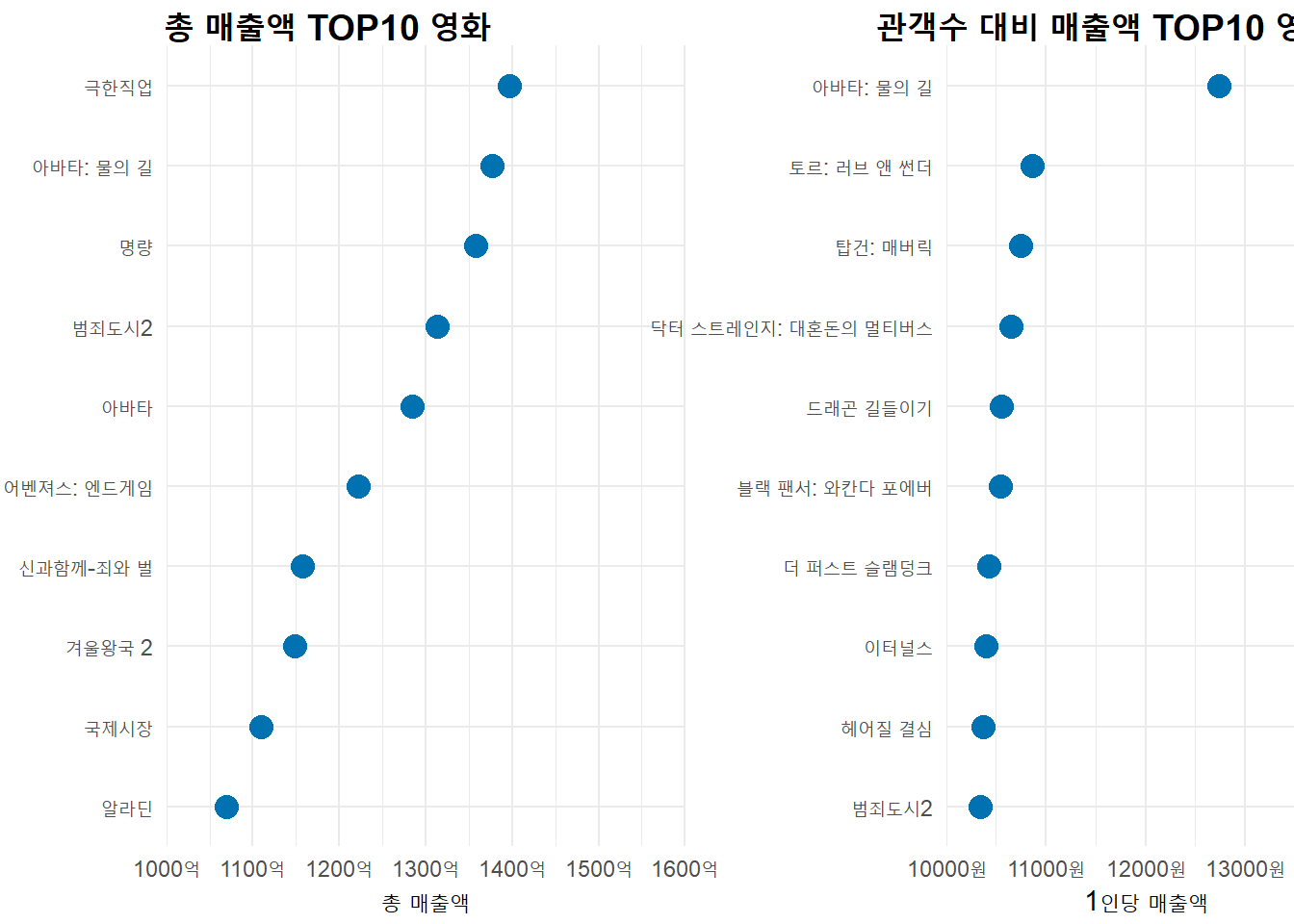
5 영화 국적별 스크린수 총합
- 전처리
con_movie <-
movie %>% group_by(국적) %>%
summarise(스크린수총합 = sum(스크린수),
매출액총합 = sum(매출액, na.rm = T))
con_movie$color <- c("#B6494A", "#000000", "#FFED00", "#E30113", "#E7D739","#4E4E4E")
con_movie
#> # A tibble: 6 × 4
#> 국적 스크린수총합 매출액총합 color
#> <chr> <dbl> <dbl> <chr>
#> 1 미국 197817 5830394959732 #B6494A
#> 2 영국 568 24982533500 #000000
#> 3 일본 2350 98086049816 #FFED00
#> 4 중국 473 17910684413 #E30113
#> 5 프랑스 936 33552487553 #E7D739
#> 6 한국 209321 7519517818134 #4E4E4E
con_movie2 <- con_movie %>%
arrange(스크린수총합) %>%
mutate(party_fac = factor(국적, levels = 국적[order(스크린수총합)]),
value = 스크린수총합,
ypos = sum(value) - (cumsum(value)-0.5*value),
mid_angle = 2*pi*(ypos/sum(value)),
hjust = ifelse(mid_angle<pi, 1, 0),
vjust = ifelse(mid_angle<pi, mid_angle/pi, 2-mid_angle/pi))
con_movie2
#> # A tibble: 6 × 10
#> 국적 스크린수총합 매출액…¹ color party…² value ypos mid_a…³ hjust vjust
#> <chr> <dbl> <dbl> <chr> <fct> <dbl> <dbl> <dbl> <dbl> <dbl>
#> 1 중국 473 1.79e10 #E30… 중국 473 4.11e5 6.28 0 0.00115
#> 2 영국 568 2.50e10 #000… 영국 568 4.11e5 6.27 0 0.00368
#> 3 프랑스 936 3.36e10 #E7D… 프랑스 936 4.10e5 6.26 0 0.00733
#> 4 일본 2350 9.81e10 #FFE… 일본 2350 4.08e5 6.24 0 0.0153
#> 5 미국 197817 5.83e12 #B64… 미국 197817 3.08e5 4.71 0 0.502
#> 6 한국 209321 7.52e12 #4E4… 한국 209321 1.05e5 1.60 1 0.509
#> # … with abbreviated variable names ¹매출액총합, ²party_fac, ³mid_angle5.1 영화 국적별 스크린수 총합
- 시각화
ggplot(con_movie2, aes(x="", y=스크린수총합, fill=party_fac)) +
  geom_bar(stat = "identity") +
  geom_text(aes(x=1, y=ypos, label=스크린수총합), color="white", size=6) +
  geom_text(aes(x=1.5, y=ypos, label=국적, hjust=hjust, vjust=vjust),
            color="black", size=0) +
  geom_text_repel(aes(label = party_fac), size = 6,
                  nudge_x = ifelse(con_movie2$party_fac == "미국", 1, 1),
                  nudge_y = ifelse(con_movie2$party_fac == "한국", -2, 1),
                  segment.color = "black",
                  force = 20,
                  segment.size = 0.6) +
  coord_polar(theta = "y", start = 0, direction = -1, clip = "off") +
  scale_fill_manual(values = con_movie2$color) +
  theme_void() +
  theme(legend.position = "none") +
  labs(title = "영화 국적별 스크린 수") +
  theme(plot.title = element_text(size = 18))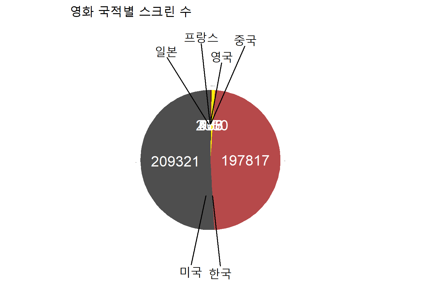
# date 형식 '개봉일' 생성
movie %>% sapply(class)
#> $순위
#> [1] "numeric"
#>
#> $영화이름
#> [1] "character"
#>
#> $개봉일
#> [1] "POSIXct" "POSIXt"
#>
#> $매출액
#> [1] "numeric"
#>
#> $관객수
#> [1] "numeric"
#>
#> $스크린수
#> [1] "numeric"
#>
#> $국적
#> [1] "character"
#>
#> $배급사
#> [1] "character"
movie$개봉일 <- movie$개봉일 %>% as.Date()
movie
#> # A tibble: 500 × 8
#> 순위 영화이름 개봉일 매출액 관객수 스크…¹ 국적 배급사
#> <dbl> <chr> <date> <dbl> <dbl> <dbl> <chr> <chr>
#> 1 1 명량 2014-07-30 135748398910 1.76e7 1587 한국 "(주)…
#> 2 2 극한직업 2019-01-23 139647979516 1.63e7 1978 한국 "(주)…
#> 3 3 신과함께-죄와 벌 2017-12-20 115698654137 1.44e7 1912 한국 "롯데…
#> 4 4 국제시장 2014-12-17 110913469630 1.43e7 966 한국 "(주)…
#> 5 5 어벤져스: 엔드게임 2019-04-24 122182694160 1.39e7 2835 미국 "월트…
#> 6 6 겨울왕국 2 2019-11-21 114810421450 1.37e7 2648 미국 "월트…
#> 7 7 아바타 2009-12-17 128447097523 1.36e7 912 미국 "주식…
#> 8 8 베테랑 2015-08-05 105168155250 1.34e7 1064 한국 "(주)…
#> 9 9 괴물 2006-07-27 0 1.30e7 167 한국 "(주)…
#> 10 10 도둑들 2012-07-25 93665568500 1.30e7 1072 한국 "(주)…
#> # … with 490 more rows, and abbreviated variable name ¹스크린수6 연도별 통계 시각화
# 관객수
movie_sum <- movie %>%
  mutate(연도 = lubridate::year(개봉일)) %>%
  group_by(연도) %>%
  summarise(총합 = sum(관객수))

movie_sum
#> # A tibble: 26 × 2
#>     연도     총합
#>    <dbl>    <dbl>
#>  1  1998  1971780
#>  2  1999  8130000
#>  3  2000  2513540
#>  4  2001  2678846
#>  5  2002 16367697
#>  6  2003 64995866
#>  7  2004 62340959
#>  8  2005 85616773
#>  9  2006 82869100
#> 10  2007 74889204
#> # … with 16 more rows

sum1_plot <-
ggplot(movie_sum, aes(x = 연도, y = 총합)) +
  geom_line(color = "royalblue", size = 1) +
  scale_x_continuous(name = "개봉연도") +
  scale_y_continuous(labels = comma, name = "관객수 총합") +
  labs(title = "연도별 관객수 총합") +
  theme_minimal()
#> Warning: Using `size` aesthetic for lines was deprecated in ggplot2 3.4.0.
#> ℹ Please use `linewidth` instead.


# 스크린수
movie_sum2 <- movie %>%
  mutate(연도 = lubridate::year(개봉일)) %>%
  group_by(연도) %>%
  summarise(총합 = sum(스크린수))

movie_sum2
#> # A tibble: 26 × 2
#>     연도  총합
#>    <dbl> <dbl>
#>  1  1998     0
#>  2  1999     0
#>  3  2000     0
#>  4  2001     0
#>  5  2002   280
#>  6  2003  1293
#>  7  2004  1412
#>  8  2005  2070
#>  9  2006  2134
#> 10  2007  2708
#> # … with 16 more rows

sum2_plot <-
ggplot(movie_sum2, aes(x = 연도, y = 총합)) +
  geom_line(color = "royalblue", size = 1) +
  scale_x_continuous(name = "개봉연도") +
  scale_y_continuous(labels = comma, name = "스크린수 총합") +
  labs(title = "연도별 스크린수 총합") +
  theme_minimal()

# 매출액
movie_sum3 <- movie %>%
  mutate(연도 = lubridate::year(개봉일)) %>%
  group_by(연도) %>%
  summarise(총합 = sum(매출액,na.rm = T))

movie_sum3
#> # A tibble: 26 × 2
#>     연도      총합
#>    <dbl>     <dbl>
#>  1  1998         0
#>  2  1999         0
#>  3  2000         0
#>  4  2001         0
#>  5  2002         0
#>  6  2003         0
#>  7  2004         0
#>  8  2005         0
#>  9  2006         0
#> 10  2007 549434500
#> # … with 16 more rows

label_억 <- function(x) {
  x <- x / 1e8
  sprintf("%.0f억", x)}  #억

sum3_plot <-
ggplot(movie_sum3, aes(x = 연도, y = 총합)) +
  geom_line(color = "royalblue", size = 1) +
  scale_x_continuous(name = "개봉연도") +
  scale_y_continuous(labels = label_억, name = "매출액 총합", expand = c(0, 0)) +
  labs(title = "연도별 매출액 총합") +
  theme_minimal()


### 2개의 temp_long 그래프
plot_2 <- plot_grid(sum1_plot,
                     sum2_plot,
                     nrow= 1,            # 행의 개수
                     rel_widths= c(1.5,1.5)) # 각각의 너비


### plot_ab 그래프 + templong 그래프
plot_abc <- plot_grid(plot_2,
                      sum3_plot,
                      ncol= 1,               # 열의 개수
                      rel_heights= c(1.5, 1))# 각각의 높이

plot_abc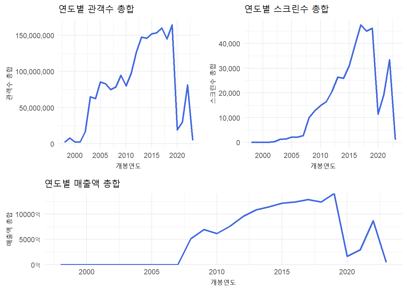
movie %>% group_by(국적)
#> # A tibble: 500 × 8
#> # Groups: 국적 [6]
#> 순위 영화이름 개봉일 매출액 관객수 스크…¹ 국적 배급사
#> <dbl> <chr> <date> <dbl> <dbl> <dbl> <chr> <chr>
#> 1 1 명량 2014-07-30 135748398910 1.76e7 1587 한국 "(주)…
#> 2 2 극한직업 2019-01-23 139647979516 1.63e7 1978 한국 "(주)…
#> 3 3 신과함께-죄와 벌 2017-12-20 115698654137 1.44e7 1912 한국 "롯데…
#> 4 4 국제시장 2014-12-17 110913469630 1.43e7 966 한국 "(주)…
#> 5 5 어벤져스: 엔드게임 2019-04-24 122182694160 1.39e7 2835 미국 "월트…
#> 6 6 겨울왕국 2 2019-11-21 114810421450 1.37e7 2648 미국 "월트…
#> 7 7 아바타 2009-12-17 128447097523 1.36e7 912 미국 "주식…
#> 8 8 베테랑 2015-08-05 105168155250 1.34e7 1064 한국 "(주)…
#> 9 9 괴물 2006-07-27 0 1.30e7 167 한국 "(주)…
#> 10 10 도둑들 2012-07-25 93665568500 1.30e7 1072 한국 "(주)…
#> # … with 490 more rows, and abbreviated variable name ¹스크린수
datetime <- as.POSIXct(movie$개봉일, format = "%Y-%m-%d %H:%M:%S")
datetime_str <- format(datetime, "%Y-%m-%d")
movie$개봉연도 <- substr(datetime_str,1,4)
movie
#> # A tibble: 500 × 9
#> 순위 영화이름 개봉일 매출액 관객수 스크…¹ 국적 배급사 개봉연도
#> <dbl> <chr> <date> <dbl> <dbl> <dbl> <chr> <chr> <chr>
#> 1 1 명량 2014-07-30 1.36e11 1.76e7 1587 한국 "(주)… 2014
#> 2 2 극한직업 2019-01-23 1.40e11 1.63e7 1978 한국 "(주)… 2019
#> 3 3 신과함께-죄와 벌 2017-12-20 1.16e11 1.44e7 1912 한국 "롯데… 2017
#> 4 4 국제시장 2014-12-17 1.11e11 1.43e7 966 한국 "(주)… 2014
#> 5 5 어벤져스: 엔드… 2019-04-24 1.22e11 1.39e7 2835 미국 "월트… 2019
#> 6 6 겨울왕국 2 2019-11-21 1.15e11 1.37e7 2648 미국 "월트… 2019
#> 7 7 아바타 2009-12-17 1.28e11 1.36e7 912 미국 "주식… 2009
#> 8 8 베테랑 2015-08-05 1.05e11 1.34e7 1064 한국 "(주)… 2015
#> 9 9 괴물 2006-07-27 0 1.30e7 167 한국 "(주)… 2006
#> 10 10 도둑들 2012-07-25 9.37e10 1.30e7 1072 한국 "(주)… 2012
#> # … with 490 more rows, and abbreviated variable name ¹스크린수
movie_group_year <-
movie %>% group_by(개봉연도) %>%
summarise(관객수총합 = sum(관객수),
스크린총합 = sum(스크린수))
movie_group_year
#> # A tibble: 26 × 3
#> 개봉연도 관객수총합 스크린총합
#> <chr> <dbl> <dbl>
#> 1 1998 1971780 0
#> 2 1999 8130000 0
#> 3 2000 2513540 0
#> 4 2001 2678846 0
#> 5 2002 16367697 280
#> 6 2003 64995866 1293
#> 7 2004 62340959 1412
#> 8 2005 85616773 2070
#> 9 2006 82869100 2134
#> 10 2007 74889204 2708
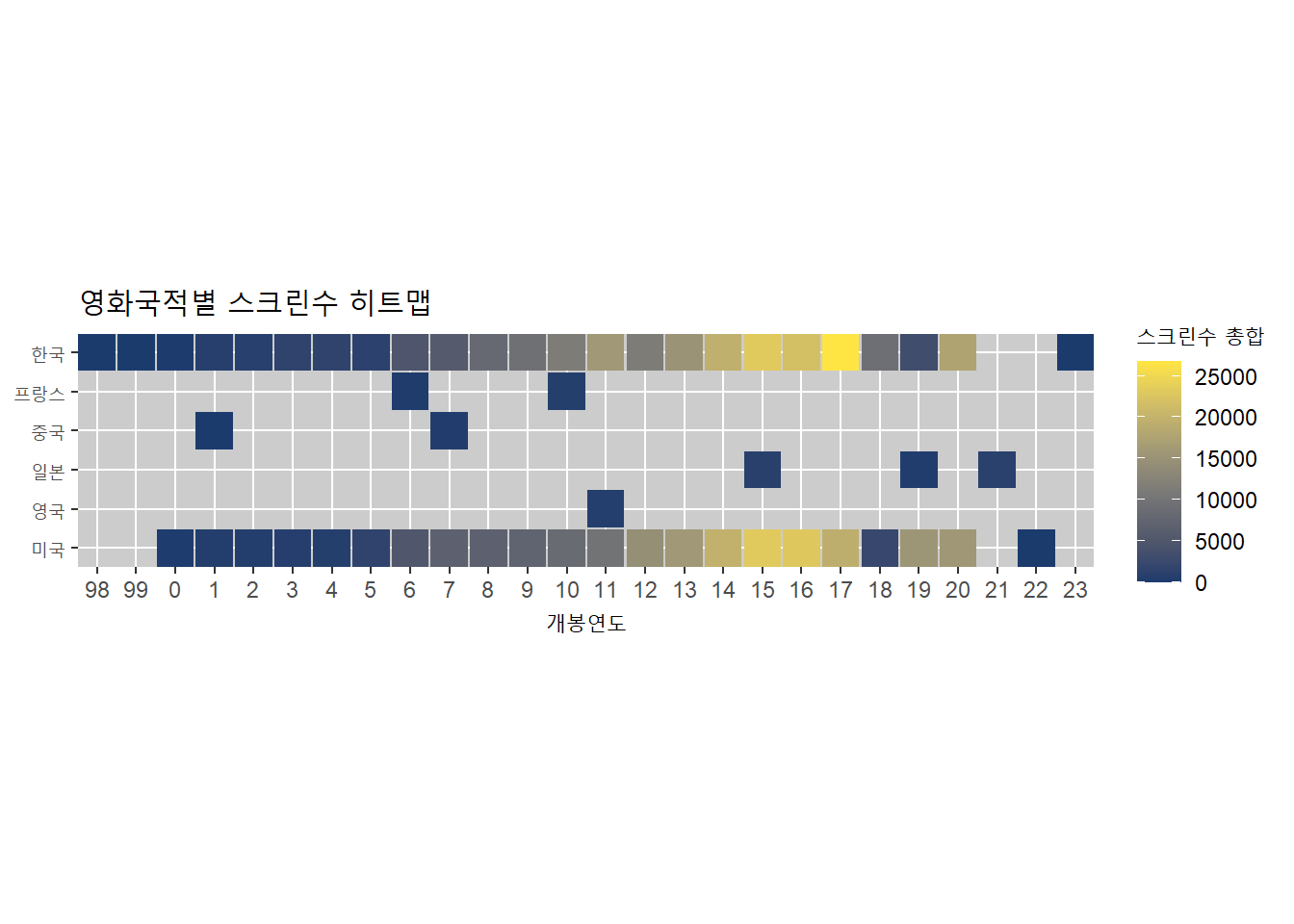
#> # … with 16 more rows7 국적별 국내 개봉 스크린 수
movie
#> # A tibble: 500 × 9
#> 순위 영화이름 개봉일 매출액 관객수 스크…¹ 국적 배급사 개봉연도
#> <dbl> <chr> <date> <dbl> <dbl> <dbl> <chr> <chr> <chr>
#> 1 1 명량 2014-07-30 1.36e11 1.76e7 1587 한국 "(주)… 2014
#> 2 2 극한직업 2019-01-23 1.40e11 1.63e7 1978 한국 "(주)… 2019
#> 3 3 신과함께-죄와 벌 2017-12-20 1.16e11 1.44e7 1912 한국 "롯데… 2017
#> 4 4 국제시장 2014-12-17 1.11e11 1.43e7 966 한국 "(주)… 2014
#> 5 5 어벤져스: 엔드… 2019-04-24 1.22e11 1.39e7 2835 미국 "월트… 2019
#> 6 6 겨울왕국 2 2019-11-21 1.15e11 1.37e7 2648 미국 "월트… 2019
#> 7 7 아바타 2009-12-17 1.28e11 1.36e7 912 미국 "주식… 2009
#> 8 8 베테랑 2015-08-05 1.05e11 1.34e7 1064 한국 "(주)… 2015
#> 9 9 괴물 2006-07-27 0 1.30e7 167 한국 "(주)… 2006
#> 10 10 도둑들 2012-07-25 9.37e10 1.30e7 1072 한국 "(주)… 2012
#> # … with 490 more rows, and abbreviated variable name ¹스크린수
movie5 <- movie %>%
mutate(year = format(개봉일, "%Y")) %>% # 일시에서 월만 뽑아낸 month 컬럼 생성
group_by(국적, year) %>% # 지점명, month로 그룹화
summarise(sum = sum(스크린수)) # 그룹화된 데이터의 집계값 요약 # 그룹화를 해제하여 일반적인 데이터 프레임 형태로 사용
#> `summarise()` has grouped output by '국적'. You can override using the
#> `.groups` argument.
# month값을 factor 형태로 수정해서 원하는 levels 지정가능 # sep='' : 간격없이 붙이기
movie5$year <- movie5$year %>% format()
movie5$개봉연도 <- substr(movie5$year,3,4)
movie5$개봉연도 <- movie5$개봉연도 %>% as.factor()
movie5
#> # A tibble: 54 × 4
#> # Groups: 국적 [6]
#> 국적 year sum 개봉연도
#> <chr> <chr> <dbl> <fct>
#> 1 미국 1998 0 98
#> 2 미국 2002 168 02
#> 3 미국 2003 505 03
#> 4 미국 2004 532 04
#> 5 미국 2005 630 05
#> 6 미국 2006 689 06
#> 7 미국 2007 1538 07
#> 8 미국 2008 4945 08
#> 9 미국 2009 6767 09
#> 10 미국 2010 6736 10
#> # … with 44 more rows
ggplot(movie5, aes(x = 개봉연도, y = 국적, fill = sum)) +
geom_tile(width = 0.95, height = 0.95) +
scale_fill_viridis_c(option = 'E', begin = 0.15, end = 0.98,
name = '스크린수 총합') +
coord_fixed(expand = FALSE) +
ylab(NULL) +
labs(title = "영화국적별 스크린수 히트맵") +
theme(panel.background = element_rect(fill = "grey80")) +
scale_x_discrete(labels = c(98,99,seq(00,23,1)))#ylab('')